3. Introduction to NumPy
An array is a way of storing several items (e.g. integers) in a single variable. Arrays are a systematic arrangement of objects, usually arranged in rows and columns. NumPy is a package for scientific computing in Python, which adds support for large multi-dimensional arrays. Arrays are similar to lists, but:
- They can be very large and multi-dimensional
- They are memory efficient, and provide fast numerical operations
- They can contain only a single data type in one array
A good example of a form of data that numpy is indispensible for is an image, such as data from an Earth Observation satellite.
The numpy module can be imported into Python with the code:
>>> import numpy
…however, because numpy is used so frequently, it is usually shortened to np by importing as:
>>> import numpy as np
3.1. Creating numpy arrays
The easiest way to create a numpy array is using a list and the np.array function:
>>> import numpy as np

>>> a = np.array([1,2,3])

>>> a
array([1, 2, 3])
Arrays can be multi-dimensional (2D, 3D, 4D…):
>>> b = np.array([[4,1,3],[7,2,5],[1,8,7]]) # A 2D array

>>> b
array([[4, 1, 3],
       [7, 2, 5],
       [1, 8, 7]])
Arrays have a number of attributes:
>>> a.ndim # Number of dimensions
1

>>> a.shape # Shape of array
(3,)

>>> b.ndim
2

>>> b.shape
(3, 3)
There are other ways to create numpy arrays:
>>> np.arange(10)
array([0, 1, 2, 3, 4, 5, 6, 7, 8, 9])

>>> np.arange(0, 50, 5) #Numbers from 0 to 50 in steps of 5
array([ 0,  5, 10, 15, 20, 25, 30, 35, 40, 45])

>>> np.linspace(10, 20, 21) #Numbers from 10 to 20, linearly split into an array of 21 elements
array([ 10. ,  10.5,  11. ,  11.5,  12. ,  12.5,  13. ,  13.5,  14. ,
    14.5,  15. ,  15.5,  16. ,  16.5,  17. ,  17.5,  18. ,  18.5,
    19. ,  19.5,  20. ])

>>> np.zeros(10)
array([ 0.,  0.,  0.,  0.,  0.,  0.,  0.,  0.,  0.,  0.])

>>> np.ones(10)
array([ 1.,  1.,  1.,  1.,  1.,  1.,  1.,  1.,  1.,  1.])

>>> np.ones((3,3))
array([[1., 1., 1.],
       [1., 1., 1.],
       [1., 1., 1.]])
You may have noticed that in some instances array elements are shown with a trailing dot (e.g. 1. vs 1). This indicates the type of numerical data held in the array (i.e. integer or float). Be aware that a numpy array can only hold one data type at once.
>>> a
array([1, 2, 3])

>>> a.dtype
dtype('int64')

>>> c = np.array([1., 2., 3.])

>>> c.dtype
dtype('float64')
3.1.1. Exercise: Array creation
- Create an array containing the numbers 1 to 100, in steps of 0.5
- Create an array containing all odd numbers from 1 to 100
- Make an array containing the integer 10, repeated 20 times
3.2. Array operations
Numpy arrays can be modified using the standard python operators:
>>> a + 1 # Adds 1 to all elements
array([ 2, 3, 4])

>>> a - 1 # Subtracts 1 from all elements
array([ 0, 1, 2])

>>> a * 5 # Multiplies all elements by 5
array([ 5, 10, 15])

>>> a / 10. # Divides all elements by 10. Why do we divide by a float here?
array([ 0.1,  0.2,  0.3])
We can also perform operations on two arrays:
>>> a * a # What's happening here?
array([1, 4, 9])

>>> b + b # What's happening here?
array([[ 8,  2,  6],
       [14,  4, 10],
       [ 2, 16, 14]])

>>> a * b # What's happening here?
array([[ 4,  2,  9],
       [ 7,  4, 15],
       [ 1, 16, 21]])
3.3. Array indexing
Much like lists, we can access the elements of an array independently. Make sure you understand what is happening in each of these examples:
>>> a[0]
1

>>> a[1]
2

>>> a[-1]
3

>>> b[1]
array([7, 2, 5])

>>> b[1,1]
2
In a similar manner to lists, arrays can also be sliced into parts:
>>> x = np.arange(100)

>>> x[10:20] # Get the elements from 10 to 20
array([10, 11, 12, 13, 14, 15, 16, 17, 18, 19])

>>> x[::10] # Get every 10th element
array([ 0, 10, 20, 30, 40, 50, 60, 70, 80, 90])

>>> y = np.random.rand(6,6) # Create a 6 by 6 array of random numbers

>>> y[:3,:3] # Select the first 3 rows and columns
array([[ 0.1545669 ,  0.35908932,  0.30732055],
       [ 0.21162311,  0.09059191,  0.87824174],
       [ 0.72614825,  0.0266589 ,  0.41946432]])
3.4. Assignment
Using similar methods, we can assign values to elements of an array
>>> y[:3,:3] = 0 # Set the first 3 rows and columns to equal 0

>>> y
array([[ 0.        ,  0.        ,  0.        ,  0.984333  ,  0.79586604,  0.99353897],
       [ 0.        ,  0.        ,  0.        ,  0.3648008 ,  0.81364244,  0.83354187],
       [ 0.        ,  0.        ,  0.        ,  0.42934255,  0.52064217,  0.25940776],
       [ 0.95443339,  0.83289332,  0.91049323,  0.71452678,  0.13792483,  0.79273019],
       [ 0.4731708 ,  0.01571735,  0.98596698,  0.95775551,  0.11409062,  0.72255358],
       [ 0.87815504,  0.60418293,  0.17141781,  0.44434767,  0.56713818,  0.53995463]])

>>> y[-1,-1] = 1 # Set the lower right array element to equal 1
array([[ 0.        ,  0.        ,  0.        ,  0.984333  ,  0.79586604,  0.99353897],
       [ 0.        ,  0.        ,  0.        ,  0.3648008 ,  0.81364244,  0.83354187],
       [ 0.        ,  0.        ,  0.        ,  0.42934255,  0.52064217,  0.25940776],
       [ 0.95443339,  0.83289332,  0.91049323,  0.71452678,  0.13792483,  0.79273019],
       [ 0.4731708 ,  0.01571735,  0.98596698,  0.95775551,  0.11409062,  0.72255358],
       [ 0.87815504,  0.60418293,  0.17141781,  0.44434767,  0.56713818,  1.]])
3.4.1. Exercise: Array manipulation
- Create the following arrays using the methods we have covered:
array([3, 2, 1])

array([  0,  20,  40,  60,  80, 100, 120, 140, 160, 180, 200, 220, 240,
         260, 280, 300, 320, 340, 360, 380, 400, 420, 440, 460, 480, 500,
         520, 540, 560, 580, 600, 620, 640, 660, 680, 700, 720, 740, 760,
         780, 800, 820, 840, 860, 880, 900, 920, 940, 960, 980])

array([[ 1.,  1.,  1.,  1.,  1.],
       [ 1.,  1.,  1.,  4.,  1.],
       [ 1.,  1.,  1.,  1.,  1.],
       [ 1.,  1.,  1.,  1.,  1.],
       [ 2.,  2.,  2.,  2.,  2.]])
- Can you make a three dimensional array of random numbers?
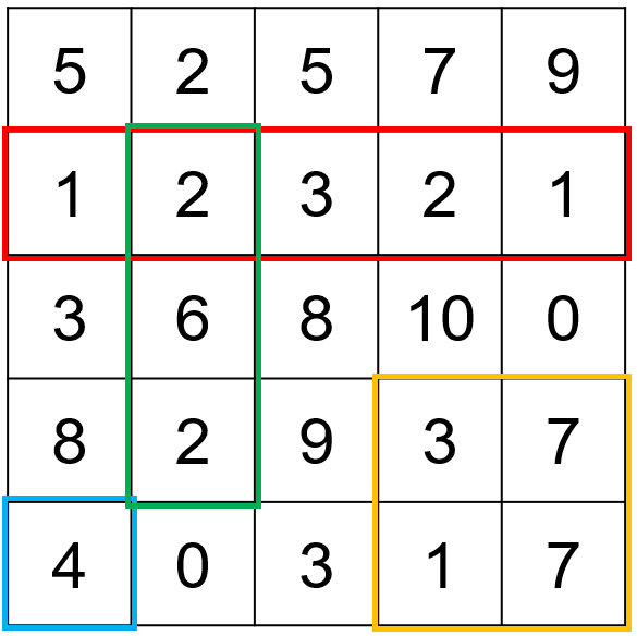
- Create the following array. Use the indexing methods to extract the four outlined areas:
3.5. Functions
Numpy includes a large number of useful functions.
Here are some examples of commonly used functions.
>>> a = np.arange(1,11)

>>> np.sum(a) # The sum total of an array
55

>>> np.min(a) # Minumum value of an array
1

>>> np.max(a) # Maxiumum value of an array
10

>>> np.mean(a) # Mean value of an array
5.5

>>> b = a.reshape(5,2) # Change the dimensions of a shape

>>> b
array([[ 1,  2],
       [ 3,  4],
       [ 5,  6],
       [ 7,  8],
       [ 9, 10]])

>>> np.sum(b, axis=0) # Sum along the vertical axis of the array
array([25, 30])

>>> np.sum(b, axis=1) # Sum along the horizontal axis of the array
array([ 3,  7, 11, 15, 19])
3.5.1. Exercise: More array manipulation
- Create the following array (in one line of code!)
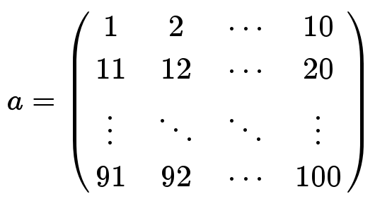
Using this array:
- Calculate the sum total of the array
- Calculate the mean of the array
- Calculate the mean of each row of the array
- Extract the 3rd row of the array (numbers 21 to 30)
3.6. Masking
For some kinds of data, it can be useful to mask (or hide) certain values. For example, cloud-covered pixels in an optical satellite image. Masks are boolean arrays (values of True and False), where values of True refer to locations that should be masked.
>>> x = np.random.rand(6,6)

>>> x > 0.5
array([[ True,  True, False, False, False, False],
       [ True, False, False,  True, False, False],
       [ True, False,  True, False,  True, False],
       [False,  True, False, False, False,  True],
       [False,  True, False, False, False, False],
       [ True, False,  True, False,  True,  True]], dtype=bool)

>>> np.logical_and(x > 0.5, x < 0.75) # Multiple conditions can be combined
array([[ True,  True, False, False, False, False],
       [False, False, False,  True, False, False],
       [ True, False, False, False,  True, False],
       [False,  True, False, False, False, False],
       [False, False, False, False, False, False],
       [False, False,  True, False, False, False]], dtype=bool)

>>> x[x > 0.9] # Extract all elements that meet given criteria
array([ 0.9354168 ,  0.91462   ,  0.98655895,  0.91459135,  0.90945349])
Since the masks are also numpy arrays, these can be stored and used to mask other arrays.
>>> mask = x > 0.9

>>> mask # Mask shows True where x > 0.9
array([[False, False, False, False, False, False],
       [ True, False, False, False, False, False],
       [False, False, False, False, False, False],
       [False, False, False, False, False,  True],
       [False,  True, False, False, False, False],
       [False, False, False, False,  True,  True]], dtype=bool)

>>> y = np.random.rand(6,6)

>>> y[mask] # Extract the values of y where x > 0.9
    array([ 0.28332556,  0.20372563,  0.15115744,  0.08839921,  0.83573746])
We can apply mutiple conditions these boolean masks using the and and or statements we looked at in the previous section. However, the syntax is a little different:
>>> mask = np.logical_or(x < 0.25, x > 0.75) # Masks everything below 0.25 and over 0.75

>>> mask = np.logical_and(x > 0.25, x < 0.75) # Masks everything over 0.25 but below 0.75
There is also a special class of numpy array known as a masked array, which we’ll look at in the next section. You can use this to store both data and a mask in one object. You can create a masked array as follows:
>>> masked_array = np.ma.array(x, mask = mask) # Creates a masked array.
3.6.1. Exercise: Looking at some real data
Here we’ll take a look at some real data from MODIS. I have extracted a time series of leaf area index (LAI) estimates every 8 days over the years 2001 - 2010 over Kilwa District in southeastern Tanzania. The data can be downloaded here: kilwaLAI.npz.
The data look like this:
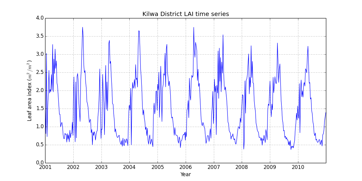
We’ll learn to make a plot like this in the next section.
First, download the data and load into Python using the following commands.
>>> data = np.load('kilwaLAI.npz') # make sure that you put the path to your copy of kilwaLAI.npz

>>> LAI = data['LAI'] # Leaf area index, units of m^2/m^2
>>> year = data['year'] # 2001 to 2010
>>> month = data['month'] # 1 to 12
Explore the data contained in these four arrays. See if you can use the functions of numpy to answer the following questions.
- What is the average LAI in Kilwa District over the whole monitoring period?
- What is the minimum and maximum LAI observed in Kilwa District?
- What proportion of the observations is LAI above 2.0?
- What was the average LAI in February 2005?
- In what months is LAI in Kilwa District at its maximum and minimum? (Hint: This is difficult. Consider using a
forloop.)